建议参考RankLib v2.1,后面的版本代码感觉有些乱:
svn co http://svn.code.sf.net/p/lemur/code/RankLib/tags/release-2.1/ Ranklib-v2.1
数据结构
- Sample -> DataPoint
- Query -> RankList
LambdaMART.java
void init()
展开RankList,初始化四个数组:
martSamples = new DataPoint[dpCount];  // 保存所有的sample
modelScores = new float[dpCount];     // 所有sample的得分
pseudoResponses = new float[dpCount];   // 所有sample的lambda值
sortedIdx = new int[features.length][];    // 临时的二维数组,保存按feature值排序后的sample id
把所有sample按照feature值排序,得到一个二维数组sortedIdx,第一维是feature id,第二维是sample id。这个步骤可以并行化:
【注】这里id都是自然数。
protected void sortSamplesByFeature(int fStart, int fEnd)
{
	for(int i=fStart;i<=fEnd; i++)
		sortedIdx[i] = sortSamplesByFeature(martSamples, features[i]);
}
以上4个数组非常吃内存,martSamples包含所有样本和特征O(mn),modelScores和pseudoResponses包含所有样本的分值O(n),sortedIdx二维数组O(mn),其中n是sample数量,m是feature维度。实际使用中,8G内存的机器只能运算几十万量级几十个维度的样本。
计算各feature的分裂点,存入二维数组thresholds:
thresholds = new float[features.length][];
计算特征直方图,用于加速节点分裂,同时释放之前的sortedIdx数组:
hist = new FeatureHistogram();
hist.construct(martSamples, pseudoResponses, sortedIdx, features, thresholds);
//we no longer need the sorted indexes of samples
sortedIdx = null;
void learn()
迭代nTrees棵树:
    computePseudoResponses();  // 计算Lambda (pseudo response),每个文档的lambda值作为training label。
    hist.update(pseudoResponses);  // 根据计算出的label更新直方图,用来下一步寻找最佳分裂节点。

    RegressionTree rt ... ; // 训练单棵回归树。
    ensemble.add(rt, learningRate);  // 把单棵树加入ensemble模型(ensemble即训练完最终的输出模型)。
    updateTreeOutput(rt);  // 更新回归树的输出(使用牛顿法估计gamma值)

    for(int i=0;i<modelScores.length;i++)  // 利用本次回归树的输出叠加样本分值(boosting)
        modelScores[i] += learningRate * rt.eval(martSamples[i]);

    scoreOnTrainingData = computeModelScoreOnTraining();  // 验证(evaluate)当前模型(计算本轮的ERR/NDCG之类的指标)
void computePseudoResponses()
计算Lambda,按Query循环,对每个RankList计算(并行化)。
// start和end是Query的下标,表示处理哪些Query;而current是Sample的下标,表示该Query的第一个sample在modelScores里的位置。
protected void computePseudoResponses(int start, int end, int current)
{
    //compute the lambda for each document (aka "pseudo response")
    for(int i=start;i<=end;i++)	{
	RankList r = samples.get(i);	// 一次Query请求返回的Sample列表
	float[][] changes = computeMetricChange(i, current);	// 计算交换顺序后的NDCG@K,changes是k*k的矩阵,其中k是本次请求的sample数量,k<=K。
	double[] lambdas = new double[r.size()];
	double[] weights = new double[r.size()];
	Arrays.fill(lambdas, 0);
	Arrays.fill(weights, 0);

	for(int j=0;j<r.size();j++) {
	    DataPoint p1 = r.get(j);
	    for(int k=0;k<r.size();k++)	{
		if(j == k)
		    continue;

		DataPoint p2 = r.get(k);
		double deltaNDCG = Math.abs(changes[j][k]);

		if(p1.getLabel() > p2.getLabel()) {
		    double rho = 1.0 / (1 + Math.exp(modelScores[current+j] - modelScores[current+k]));
		    double lambda = rho * deltaNDCG;  // lambda是ρΔNDCG,代表重排序后的指标变化
		    lambdas[j] += lambda;
		    lambdas[k] -= lambda;
		    double delta = rho * (1.0 - rho) * deltaNDCG;  // delta是lambda的偏导数
		    weights[j] += delta;
		    weights[k] += delta;
		}
	    }
	}
	// 保存每个sample的计算结果
	for(int j=0;j<r.size();j++)	{
	    pseudoResponses[current+j] = (float)lambdas[j];
	    r.get(j).setCached(weights[j]);  // 暂存起来用于后续计算gamma值
	}
	// 更新current下标
	current += r.size();
    }
}
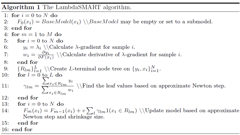
void updateTreeOutput(RegressionTree rt)
每个叶子节点上的output值即gamma。
第m轮迭代,第l个叶子节点的gamma值:
\[\gamma_{lm} = {\sum_{x_i \in R_{lm}} y_i \over \sum_{x_i \in R_{lm}} w_i}\]其中,$y_i$是样本i的lambda值,而$w_i$是$y_i$的偏导数。
gamma的含义可以参考GBDT论文 4.5 Two-class logistic regression and classification,是求解最大似然函数,用牛顿法推导出来的。
float computeModelScoreOnTraining()
评价函数。评价指标可以是MAP、ERR、NDCG等等。
遍历每次Query,根据最新的得分(modelScores)把RankList重新排序,然后算一下本次Query的排序指标得分。最后把这些得分平均一下输出。
FeatureHistogram.java
主要思路就是sample先按feature值排序好,然后算好threshold,再根据threshold分段预处理sample数据(比如每个threshold两侧的样本数、label之和、label平方之和以及各sample对应的阈值id)。
处理完的结果可用于分裂节点(寻找feature和对应的threshold),参考FeatureHistogram.findBestSplit函数。
void construct(DataPoint[] samples, float[] labels, int[][] sampleSortedIdx, int[] features, float[][] thresholds)
// feature数 x threshold数,保存阈值左侧所有sample label之和(注意左侧所有,不是与前一阈值之间)
sum = new double[features.length][];
// feature数 x threshold数,类似sum保存的是左侧label平方之和
sqSum = new double[features.length][];
//  feature数 x threshold数,保存的是左侧sample的数量
count = new int[features.length][];
// feature数 x sample数,保存的是每个sample对应的阈值id
sampleToThresholdMap = new int[features.length][];
void update(float[] labels)
输入:所有sample的当前label值(pseudo responses)。
// 遍历sample和feature
for(int k=0;k<labels.length;k++)
{
	for(int f=0;f<features.length;f++) {
		// 根据sampleToThresholdMap可以得到每个sample对应的阈值id
		int t = sampleToThresholdMap[f][k];
		// 根据新的label更新sum和sqSum
		sum[f][t] += labels[k];
		sqSum[f][t] += labels[k]*labels[k];
	}
}
Split findBestSplit(Split sp, DataPoint[] samples, float[] labels, int minLeafSupport)
输入:Split节点、所有的sample数组、所有sample当前label值、叶节点里最少sample数 输出:分裂完的Split节点(feature / threshold / avgLabel 和左右子节点)
这里会用到construct()和update()创建的若干数组(即预先计算好的不同阈值两侧的sum和sqSum等值)避免重复计算。
【注】输入参数samples和labels是全局的总体samples数组,是起到正排数据的作用。因为参数sp里的Split.samples变量保存只是全局samples的id索引,需要这两份正排数据去获取到实际的信息。
// Find the best <feature, threshold> that split the set of samples into two subsets with the smallest S (mean squared error):
// S = sum_{samples put to the left}^{(label - muLeft)^2} + sum_{samples put to the right}^{(label - muRight)^2}
// and split the input tree node using this <feature, threshold> pair.

foreach(feat: features):
	foreach(thre: thresholds):
		// 如果某个threshold之间的samples数量少于minLeafSupport,则跳过该threshold。
		countLeft // 左侧的sample数
		countRight // 右侧的sample数
		sumLeft // 左侧sample的label值之和
		sumRight // 右侧sample的label值之和
		sqSumLeft // 左侧sample的label值平方之和
		sqSumRight // 右侧sample的label值平方之和
		double varLeft = sqSumLeft - sumLeft * sumLeft / countLeft;
		double varRight = sqSumRight - sumRight * sumRight / countRight;
		double S = varLeft + varRight;   // minimize MSE
		// 寻找最小的S,并记录此时的feature id和threshold id。

// 得到最佳分裂的feature和threshold后,设置该Split节点的feature、threshold和deviance。

// 根据该feature的threshold把父节点的samples分裂成左右两份samples数组。

// 根据父节点的feature histogram,以及左右samples和对应的labels创建左右feature histogram。

// 创建该Split节点的左右子节点(根据samples、feature histogram、variance和sum)。

// 返回该Split节点。
关键是如何分裂节点。这里算的S应该是MSE,最小化MSE是分裂标准。
RegressionTree.java
void fit()
关键是insert()函数,总是把deviance最大的Split节点插入到queue的最前面。
每次也是从queue的开头取Split节点,进行分裂。这样保证总是分裂deviance最大的节点。 这里deviance即MSE,MSE大说明要做决策划分(label有偏差);如果MSE为0,那该节点就不需要分裂了。
当所有节点达到minLeafSupport数量时,停止分裂,并返回所有的叶子节点(Split.featureID==-1)。
【注】最后的回归树,其实我们只关心叶子节点,因为叶子节点保存了:
- 分裂到该叶子下的所有sample,训练过程中
updateTreeOutput时候会用到; - 该叶子的feature/threshold,预测过程会用到。
Ensemble.java
如何使用模型呢?参考 Ensemble.eval() 函数,实际就是把各颗树的output累加起来,得到最终的分值。
public float eval(DataPoint dp)
{
	float s = 0;
	for(int i=0;i<trees.size();i++)
		s += trees.get(i).eval(dp) * weights.get(i);
	return s;
}
MART.java
派生LambdaMART,关键函数有俩:
- computePseudoResponses 计算训练回归树的y
- updateTreeOutput 设置回归树叶节点的输出值
void computePseudoResponses()
MART直接使用样本的原始label和预测label的差值(残差),而不是lambda梯度。
for(int i=0;i<martSamples.length;i++)
	pseudoResponses[i] = martSamples[i].getLabel() - modelScores[i];
void updateTreeOutput(RegressionTree rt)
这里输出的是残差均值。
论文
- MART (Multiple Additive Regression Trees, a.k.a. Gradient boosted regression tree): J.H. Friedman. Greedy function approximation: A gradient boosting machine. Technical Report, IMS Reitz Lecture, Stanford, 1999; see also Annals of Statistics, 2001.
- RankNet: C.J.C. Burges, T. Shaked, E. Renshaw, A. Lazier, M. Deeds, N. Hamilton and G. Hullender. Learning to rank using gradient descent. In Proc. of ICML, pages 89-96, 2005.
- RankBoost: Y. Freund, R. Iyer, R. Schapire, and Y. Singer. An efficient boosting algorithm for combining preferences. The Journal of Machine Learning Research, 4: 933-969, 2003.
- AdaRank: J. Xu and H. Li. AdaRank: a boosting algorithm for information retrieval. In Proc. of SIGIR, pages 391-398, 2007.
- Coordinate Ascent: D. Metzler and W.B. Croft. Linear feature-based models for information retrieval. Information Retrieval, 10(3): 257-274, 2007.
- LambdaMART: Q. Wu, C.J.C. Burges, K. Svore and J. Gao. Adapting Boosting for Information Retrieval Measures. Journal of Information Retrieval, 2007.
- ListNet: Z. Cao, T. Qin, T.Y. Liu, M. Tsai and H. Li. Learning to Rank: From Pairwise Approach to Listwise Approach. ICML 2007.
- Random Forests: L. Breiman. Random Forests. Machine Learning 45 (1): 5–32, 2001.